
18. Important Graphs
Free Economy rapid revision notes for UPSC, APPSC and TGPSC. Original notes are presented below with their tables, images and visual aids preserved.
18. Important Graphs
Each graph below comes with a short guide on how to read it and the exam point to remember. In every diagram, the horizontal axis (x) and the vertical axis (y) are labelled, so check what they show before reading the curve.
1. Production Possibility Frontier (PPF)
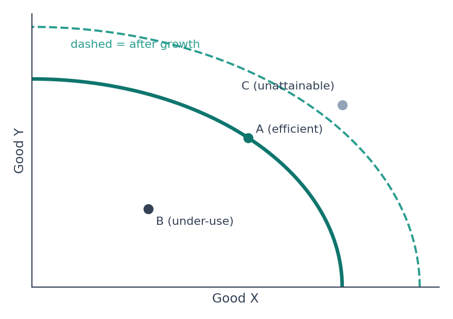
Shows the maximum combinations of two goods an economy can produce with its resources and technology.
Points on the curve are efficient; points inside show unused resources; points outside are unattainable.
Economic growth shifts the PPF outward. It is concave because of rising opportunity cost.
2. Demand and Supply: Equilibrium
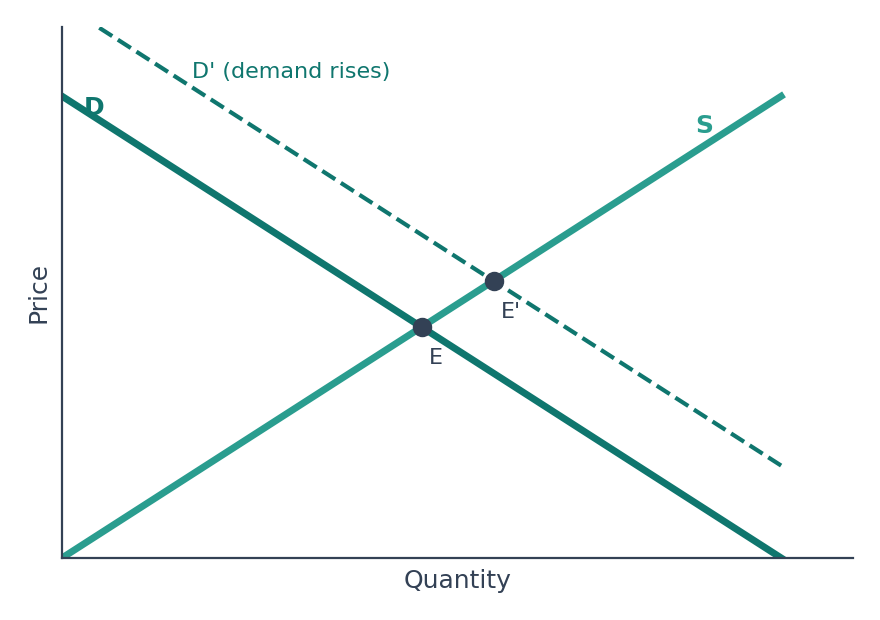
Equilibrium E is where demand equals supply, giving the market price and quantity.
A rise in demand shifts the demand curve right; both price and quantity rise (E to E').
A rise in supply shifts the supply curve right; price falls and quantity rises.
3. Price Floor (like MSP)
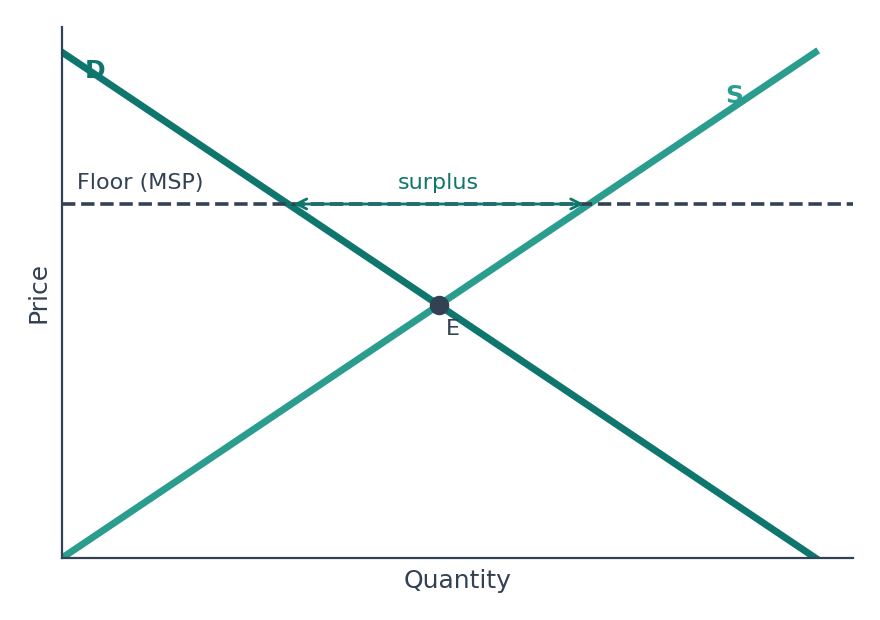
A minimum price set above equilibrium.
Supply exceeds demand, creating a surplus that the Government must buy or store.
This is why the Food Corporation of India holds large grain stocks under MSP.
4. Price Ceiling
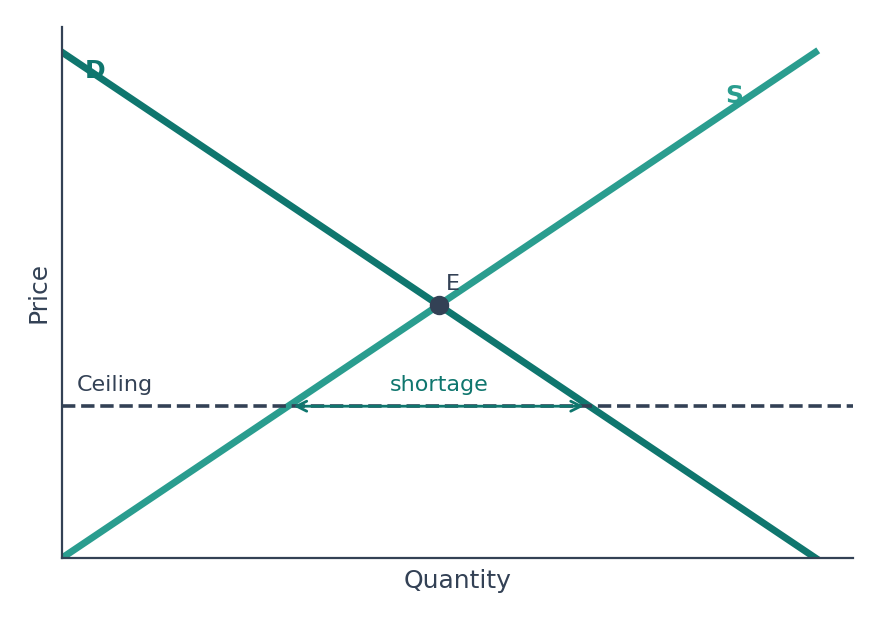
A maximum price set below equilibrium (rent control, price control on essentials).
Demand exceeds supply, creating a shortage, queues and black markets.
Intended to protect consumers, but it can reduce supply.
5. Giffen Good
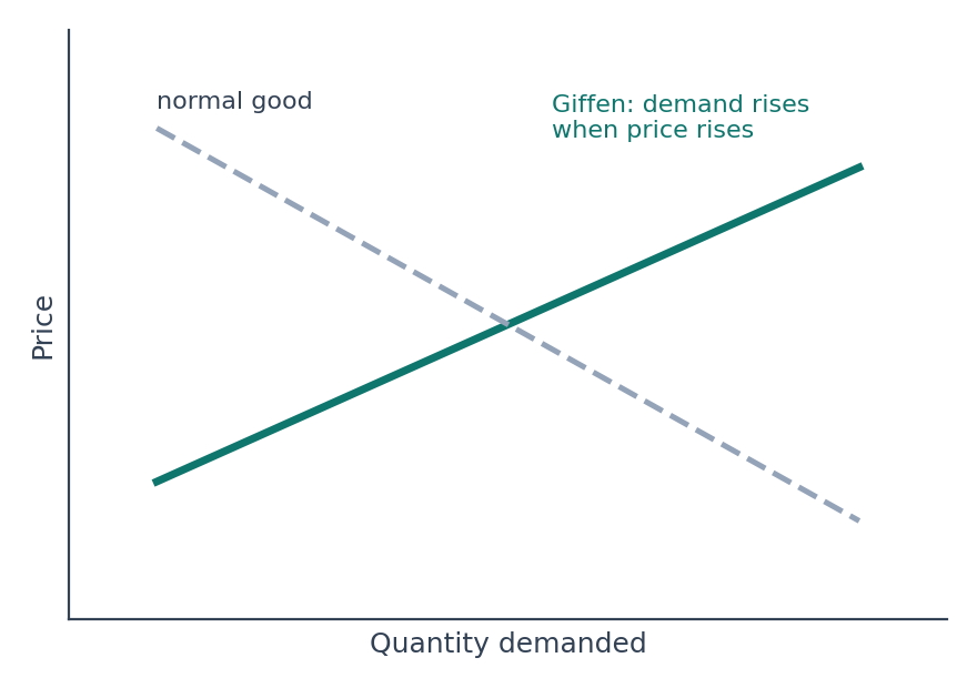
The demand curve slopes upward: demand rises as price rises.
Applies to a poor household's staple inferior good, where the income effect outweighs the substitution effect.
Named after Robert Giffen; Veblen goods also show a rising demand curve, for status reasons.
6. Lorenz Curve and Gini Coefficient
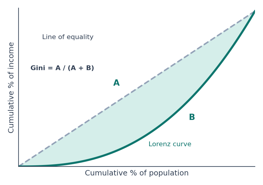
The farther the Lorenz curve is from the line of equality, the greater the inequality.
Gini = A ÷ (A + B); 0 means perfect equality and 1 means complete inequality.
Used with the Palma ratio to compare income inequality.
7. Phillips Curve
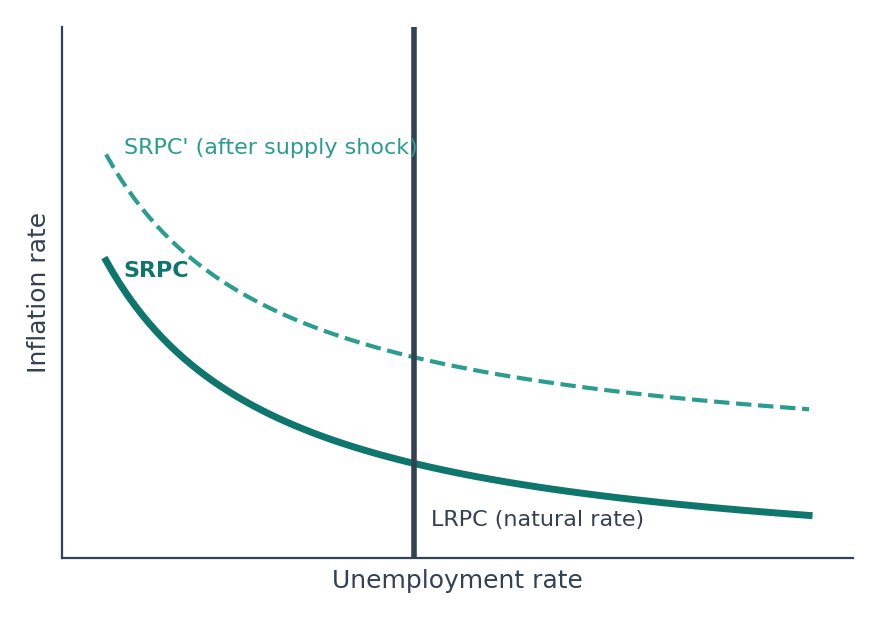
In the short run, lower unemployment goes with higher inflation (a trade-off).
In the long run the curve is vertical at the natural rate of unemployment.
Stagflation in the 1970s shifted the curve outward, which challenged the idea of a stable trade-off.
8. Laffer Curve
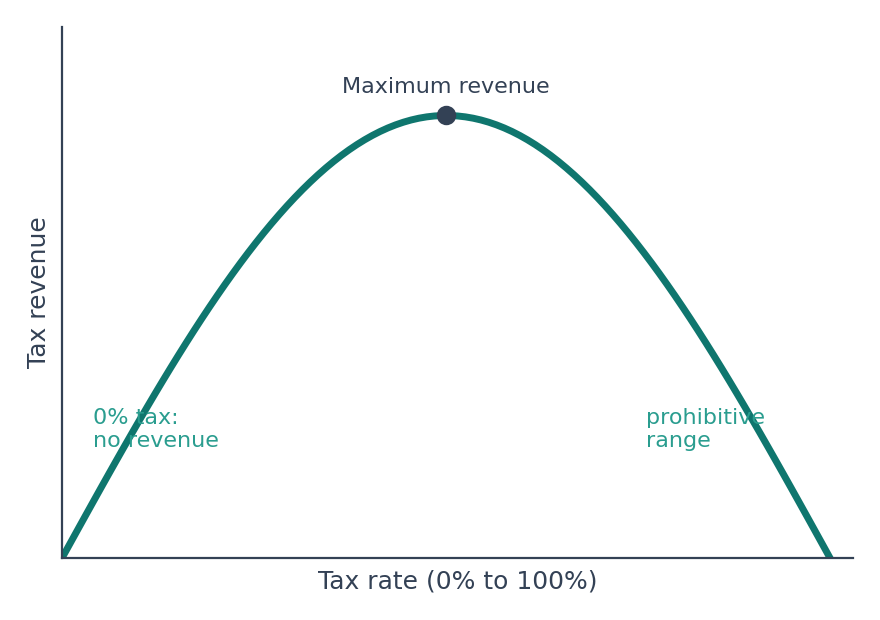
Tax revenue first rises with the tax rate, then falls after a point because people work, earn and declare less.
At 0% and at 100%, revenue is zero.
Used to argue that very high tax rates can reduce revenue.
9. Kuznets Curve
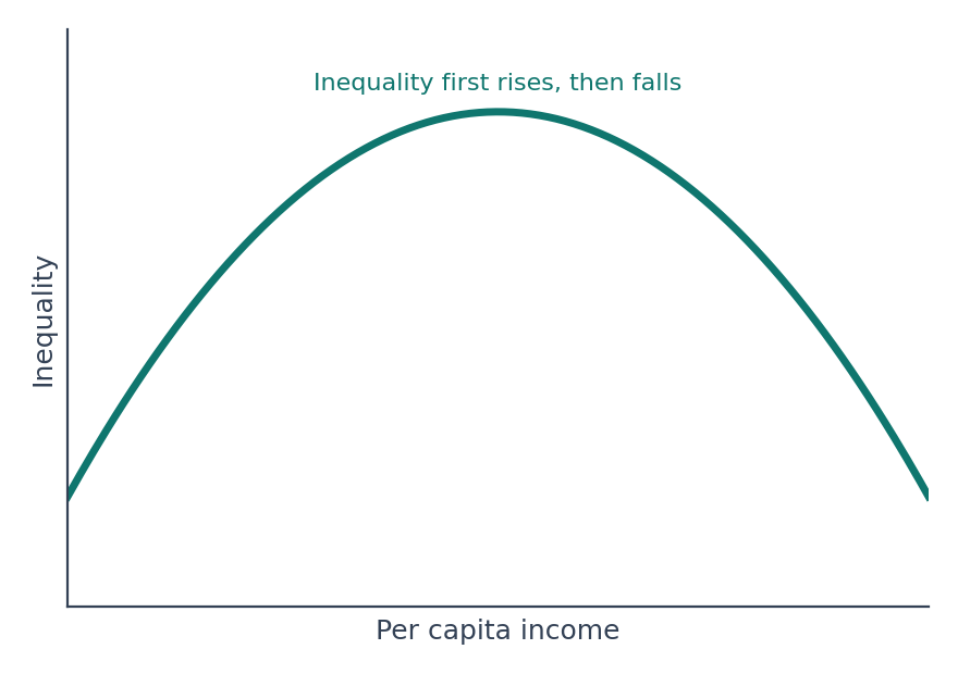
An inverted-U: inequality rises in the early stages of development and falls later as income grows.
Proposed by Simon Kuznets.
An environmental version links pollution to income in the same way.
10. J-Curve
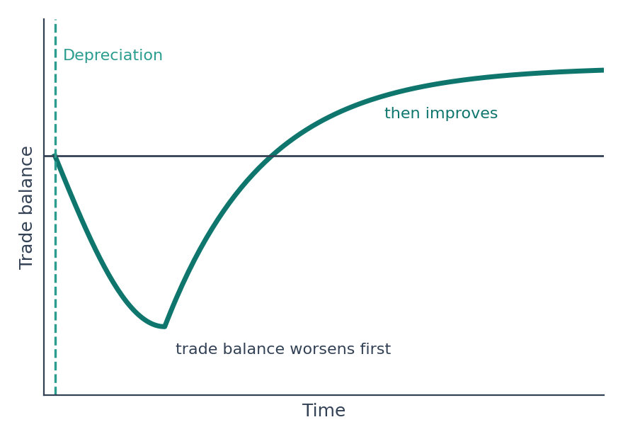
After a currency depreciates, the trade balance often worsens first because import and export contracts adjust slowly.
Later, exports rise and imports fall, so the balance improves.
Linked to the Marshall-Lerner condition.
11. Business Cycle
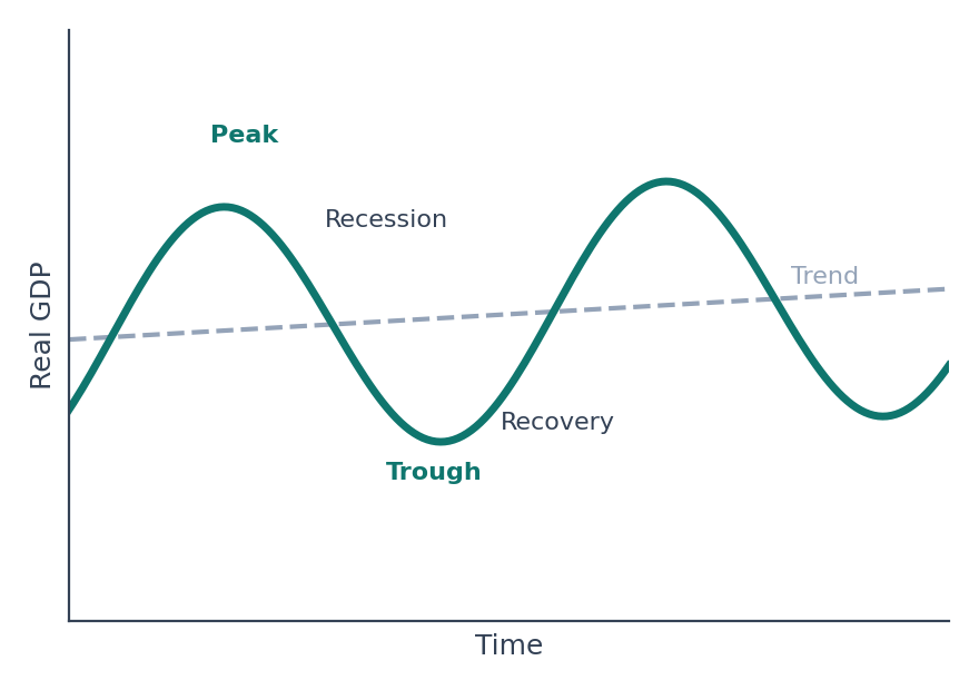
Phases: expansion (recovery), peak, recession (contraction) and trough.
Output moves around a long-run trend.
A recession is usually seen as a fall in real GDP for two or more consecutive quarters.
12. AD-AS and Stagflation
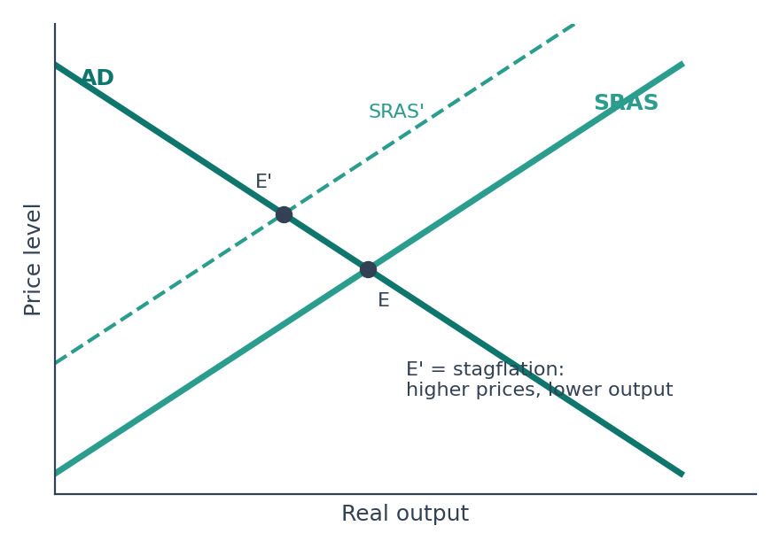
Where AD meets SRAS gives the price level and output.
A leftward shift of SRAS (from a rise in oil or input costs) raises prices and cuts output: stagflation.
A rightward shift of AD (more demand) raises both prices and output: demand-pull inflation.
13. Yield Curve
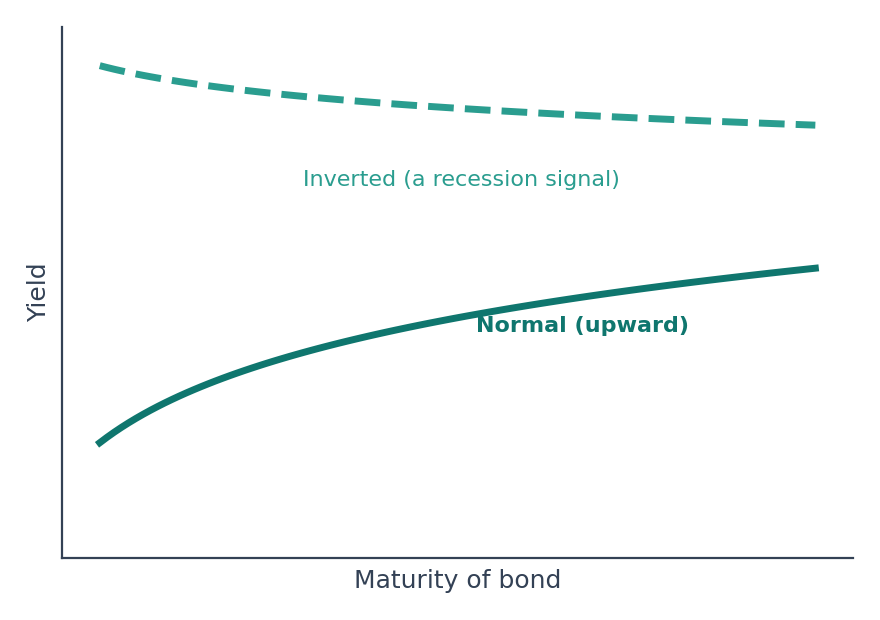
Plots the yield on bonds of different maturities.
Normal curve: slopes upward; investors need higher returns for lending longer.
Inverted curve: short-term yields exceed long-term yields; often seen as a recession signal.
14. Bond Price and Yield
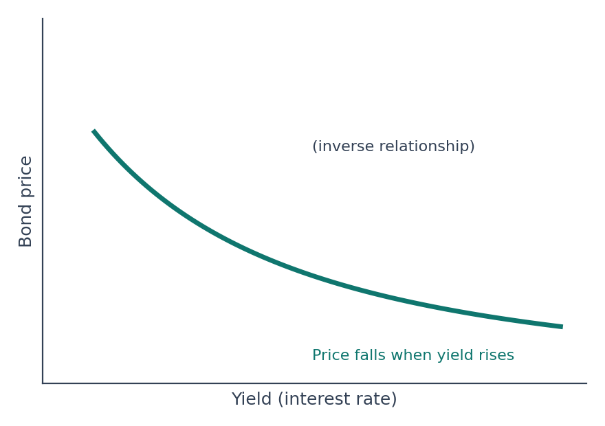
Bond prices and yields move in opposite directions.
When market interest rates rise, the price of existing bonds with lower coupons falls.
A central bank that raises rates therefore reduces bond prices.
Quick Recall
PPF: concave; growth shifts it outward; points inside show unused resources.
Price floor above equilibrium creates a surplus (MSP); price ceiling below equilibrium creates a shortage.
Giffen good: an upward-sloping demand curve.
Lorenz curve: Gini = A ÷ (A + B).
Phillips curve: short-run trade-off between inflation and unemployment; long-run vertical.
Laffer curve: an inverted U of tax revenue against tax rate.
Kuznets curve: inequality rises, then falls, with income.
J-curve: the trade balance worsens before it improves after depreciation.
Inverted yield curve: a recession signal.
Explore structured courses and guidance for your target examination.